TL;DR

I covered a brief introduction to XGBoost in the SMU Master of Professional Accounting program' elective course Programming with Data. This post is to provide an example to explain how to tune the hyperparameters of package:xgboost using the Bayesian optimization as developed in the ParBayesianOptimization package. I also demonstrate how parallel computing can save your time and computing resources.

Hyperparameter vs. parameter

I will start with a package:xgboost model with default hyperparameter values.

What? What is hyperparameter?

You must have heard about parameters such as \(\alpha\) and \(\beta\) in the ordinary least square (OLS) and Logistic regression models. So what is hyperparameter and what is the difference from parameter?

• hyperparameter: a parameter which needs to be specified before we train the model, such as lamda in the LASSO model and learing rate in the XGBoost model. These parameters will be used to control the machine learning process.
• parameter: the coefficient/weight to be derived from machines learning process, such as \(\alpha\) and \(\beta\) in the OLS regression

Did you notice that we don’t have to specify any hyperparameter when we employ the OLS and the normal Logistic models as they don’t have any hyperparameters. However, for more complex machine learning models such as LASSO, Random Forest and XGBoost, we need to specify some hyperparameters before we run the models.

For XGBoost, all the hyperparameters are available here. You may note that all those hyperparametes have default values which come with the XGBoost package. It means that if you don’t specify any new values, the model will use the default values to control the training process. If you want to change the values of hyperparameters, you need to specify them before training the model. This process is called hyperparameter tuning in the machine learning lingo.

Then why do we need to tune the hyperparameters? A simple and intuitive answer is to fine tune your model which can better train your model and hence produce better results. When you buy your mobile phone, you’d like to choose color, size and capacity. It is the same logic when you try to run complex machine learning models. So one configuration does not fit all.

XGBoost with default hypterparameter values

We will use the following packages: package:xgboost and package:ParBayesianOptimization. Both are available on the CRAN package depository which can be installed directly from RStudio or the install.packages() function.

library(xgboost)
library(ROCR)
library(ggplot2)
library(ParBayesianOptimization)

The data I will be using is a proprietary dataset of class action lawsuit. Our objective is to predict the class action lawsuit binary outcome which takes value of 1 for a class action lawsuit and 0 for none. It is labeled as legal in the dataset. So this is a typical binary classification problem. The features include companies' financial information and non-financial information such as the readability of annual report.

As I mentioned in class, if your data is large, you should use the fread() which is much faster than the read.csv(). You need to install package:data.table before running the following code.

training <- data.table::fread("training.csv")
testing <- data.table::fread("testing.csv")

Let’s first define the formula as follows. As my focus of this post is not to explain the data, I will skip data exploration. You would be able to guess what each feature means from its name.

# Equation for the regression.  -1 removes the intercept
eq = as.formula("legal ~ adj_return_FY + volume_FY + std_ret_FY +
                skew_ret_FY + log_size + growth + fps +
                Coleman_Liau_Index + Gunning_Fog_Index + 
                averageWordsPerSentence + WordCount + 
                FinTerms_Negative + FinTerms_Positive + 
                FinTerms_Litigious + FinTerms_Uncertainty - 1")

Next, we need to prepare the x data (predictors) and the y data (prediction or label) which meet the format requirement for package:xgboost. XGBoost also has its own data format using xgb.DMatrix() which I will use later.

# Make matrices for training data
x <- model.matrix(eq, data = training)
y <- model.frame(eq, data = training)[ , "legal"]

# Make matrices for testing data
xvals <- model.matrix(eq, data = testing)
yvals <- model.frame(eq, data = testing)[ , "legal"]

Now we are ready to try the XGBoost model with default hyperparameter values. We look at the following six most important XGBoost hyperparameters:

• max_depth [default=6]: Maximum depth of a tree. Increasing this value will make the model more complex and more likely to overfit. Range: [0,∞]
• eta [default=0.3]: The learning rate. Range: [0,1]
• gamma [default=0]: Minimum loss reduction required to make a further partition on a leaf node of the tree. The larger gamma is, the more conservative the algorithm will be. Range: [0,∞]
• min_child_weight [default=1]: Minimum number of observations needed in a child node. The larger min_child_weight is, the more conservative the algorithm will be. Range: [0,∞]
• subsample [default=1]: Subsample ratio of the training instances (observations). Setting it to 0.5 means that XGBoost would randomly sample half of the training data prior to growing trees. The default is 1 which means no subsample process. Subsampling will occur once in every boosting iteration. It is used to minimize the overfitting problem. Range: (0,1]
• nfold: number of cross validation (CV) folds. There is no default value and we start with the typical 10 folds cross validation. We will tune it with the range of 3 to 10 later. As this is for CV only, I will define it in the xgb.cv() function.

In addition to the above six parameters, we also specify the following hyperparameters:

• booster [default=gbtree]: tree-based boosting method. This can be used for both classification and regression problems.
• objective [default=reg:squarederror]: loss function, the default is for OLS. We will use binary:logistic for binary classification
• eval_metric [default according to objective]: Evaluation metrics for validation data, a default metric will be assigned according to objective (rmse for regression, and logloss for classification, mean average precision for ranking). We will use auc for binary classification
• verbosity [default=1]: printing messages while training the model, 0 (silent, ie,not showing any message), 1 (warning), 2 (info), 3 (debug)

The following code specifies the default value for each hyperparameter. We will try to tune these hyperparameters later.

set.seed(2021)
# The first five params to be tuned are set to default values
params <- list(max_depth = 6,
               eta = 0.3,
               gamma = 0,
               min_child_weight = 1,
               subsample = 1,

               booster = "gbtree",
               objective = "binary:logistic",
               eval_metric = "auc",
               verbosity = 0)

To minimize the overfitting problem, we use the cross validation (CV) function xgb.cv() to find out the best number of rounds (boosting iterations) for XGBoost. We use 10-fold cross validation for 100 rounds with evaluation matrix of AUC. The optimal number of rounds is determined by the minimum number of rounds which can produce the highest validation AUC (ie, lowest validation error).

The following are additional parameters for xgb.cv():

• nrounds: the max number of boosting iterations
• prediction: return the test fold predictions from each CV model
• showsd: show standard deviation of cross validation
• early_stopping_rounds: CV will stop if the performance not improve for the specified rounds
• maximize: maximize the performance for early_stopping_rounds
• stratified: a boolean indicating whether sampling of folds should be stratified by the values of outcome labels (ie, the same distribution).

xgbCV <- xgb.cv(params = params,
                data = x,
                label = y,
                nrounds = 100,
                prediction = TRUE,
                showsd = TRUE,
                early_stopping_rounds = 10,
                maximize = TRUE,
                nfold = 10,
                stratified = TRUE)

## [1]	train-auc:0.608586+0.055258	test-auc:0.572297+0.068084 
## Multiple eval metrics are present. Will use test_auc for early stopping.
## Will train until test_auc hasn't improved in 10 rounds.
## 
## [2]	train-auc:0.678191+0.033688	test-auc:0.650105+0.079131 
## [3]	train-auc:0.719241+0.006678	test-auc:0.698039+0.059299 
## [4]	train-auc:0.759246+0.042095	test-auc:0.719033+0.051714 
## [5]	train-auc:0.790659+0.025629	test-auc:0.754845+0.058458 
## [6]	train-auc:0.813285+0.019499	test-auc:0.763808+0.066096 
## [7]	train-auc:0.833346+0.023242	test-auc:0.774066+0.069199 
## [8]	train-auc:0.854651+0.020619	test-auc:0.779899+0.071212 
## [9]	train-auc:0.872086+0.020359	test-auc:0.783353+0.057533 
## [10]	train-auc:0.899344+0.005392	test-auc:0.805547+0.051509 
## [11]	train-auc:0.912967+0.005048	test-auc:0.806929+0.043305 
## [12]	train-auc:0.920942+0.005632	test-auc:0.808565+0.042629 
## [13]	train-auc:0.935232+0.009637	test-auc:0.808077+0.052455 
## [14]	train-auc:0.954605+0.006817	test-auc:0.795913+0.054406 
## [15]	train-auc:0.965291+0.004774	test-auc:0.799948+0.046381 
## [16]	train-auc:0.976118+0.005211	test-auc:0.795866+0.039994 
## [17]	train-auc:0.981229+0.004516	test-auc:0.791373+0.037651 
## [18]	train-auc:0.985593+0.003656	test-auc:0.805069+0.042414 
## [19]	train-auc:0.988762+0.002436	test-auc:0.807052+0.043763 
## [20]	train-auc:0.991113+0.002288	test-auc:0.804686+0.049946 
## [21]	train-auc:0.992633+0.001731	test-auc:0.809471+0.047058 
## [22]	train-auc:0.994259+0.001353	test-auc:0.805859+0.045883 
## [23]	train-auc:0.995357+0.001078	test-auc:0.806442+0.046140 
## [24]	train-auc:0.996342+0.000797	test-auc:0.800382+0.046470 
## [25]	train-auc:0.997282+0.000579	test-auc:0.802973+0.049742 
## [26]	train-auc:0.997959+0.000565	test-auc:0.802661+0.053013 
## [27]	train-auc:0.998488+0.000446	test-auc:0.798695+0.055943 
## [28]	train-auc:0.998864+0.000299	test-auc:0.797324+0.057295 
## [29]	train-auc:0.999128+0.000299	test-auc:0.794634+0.059362 
## [30]	train-auc:0.999378+0.000281	test-auc:0.793525+0.061460 
## [31]	train-auc:0.999553+0.000221	test-auc:0.789565+0.061613 
## Stopping. Best iteration:
## [21]	train-auc:0.992633+0.001731	test-auc:0.809471+0.047058

numrounds <- min(which(xgbCV$evaluation_log$test_auc_mean == 
                         max(xgbCV$evaluation_log$test_auc_mean)))

Finally, we can fit the XGBoost model as follows.

fit <- xgboost(params = params,
               data = x,
               label = y,
               nrounds = numrounds)

## [1]	train-auc:0.649467 
## [2]	train-auc:0.718068 
## [3]	train-auc:0.718619 
## [4]	train-auc:0.796286 
## [5]	train-auc:0.797473 
## [6]	train-auc:0.861141 
## [7]	train-auc:0.861677 
## [8]	train-auc:0.867764 
## [9]	train-auc:0.880949 
## [10]	train-auc:0.892904 
## [11]	train-auc:0.903122 
## [12]	train-auc:0.915757 
## [13]	train-auc:0.921750 
## [14]	train-auc:0.931584 
## [15]	train-auc:0.953188 
## [16]	train-auc:0.964687 
## [17]	train-auc:0.975628 
## [18]	train-auc:0.980401 
## [19]	train-auc:0.982171 
## [20]	train-auc:0.984214 
## [21]	train-auc:0.988682

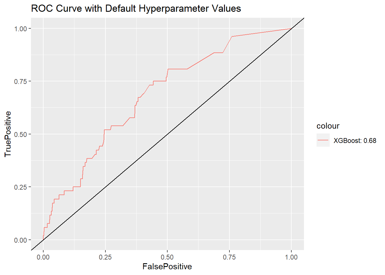
How does this model work for the testing data? Let’s compute the AUC using the package:ROCR. The value of AUC using default hyperparameter values is 0.68, which is not bad.

pred.xgb <- predict(fit, xvals, type = "response")
ROCpred.xgb <- prediction(as.numeric(pred.xgb), as.numeric(yvals))
auc.xgb <- performance(ROCpred.xgb, measure = "auc")
auc <- auc.xgb@y.values[[1]]
names(auc) <- c("XGBoost AUC")
auc

## XGBoost AUC 
##   0.6836743

We can also plot the curve.

ROCperf.xgb <- performance(ROCpred.xgb, 'tpr','fpr')
df_ROC.xgb <- data.frame(FalsePositive = c(ROCperf.xgb@x.values[[1]]),
                         TruePositive = c(ROCperf.xgb@y.values[[1]]))
ggplot() +
  geom_line(data = df_ROC.xgb, aes(x = FalsePositive,
                                   y = TruePositive,
                                   color = "XGBoost: 0.68")) + 
  geom_abline(slope = 1) +
  ggtitle("ROC Curve with Default Hyperparameter Values")

Hyperparameter tuning with bayesian optimization

The above model uses all default values of hyperparameters and the AUC is 0.68. The next question is: can we change the parameter values and achieve better results? Intuitively, we can manually try different values using for loops and compare the results (pick the one with lowest validation error) like this post. There is also packages which can help to automate this grid search process such as the package:MLR.

This process is in fact an optimization problem: minimize the validation errors. Instead of manual grid search, We can use optimization algorithm to search for the best parameter values. This is what the package:ParBayesianOptimization is trying to do.

Let me walk you through the optimization process. Please note that I typically don’t use capital letters for variable names but the package:ParBayesianOptimization defines a lot of objects using capital letters.

Define an optimizing function

This optimization function will take the tuning parameters as input and will return the best cross validation results (ie, the highest AUC score for this case). The package:ParBayesianOptimization uses the Bayesian Optimization.

In the following code, I use the XGBoost data format function xgb.DMatrix() to prepare the data.

scoring_function <- function(
  eta, gamma, max_depth, min_child_weight, subsample, nfold) {

  dtrain <- xgb.DMatrix(x, label = y, missing = NA)

  pars <- list(
    eta = eta,
    gamma = gamma,
    max_depth = max_depth,
    min_child_weight = min_child_weight,
    subsample = subsample,

    booster = "gbtree",
    objective = "binary:logistic",
    eval_metric = "auc",
    verbosity = 0
  )
  
  xgbcv <- xgb.cv(
    params = pars,
    data = dtrain,
    
    nfold = nfold,
    
    nrounds = 100,
    prediction = TRUE,
    showsd = TRUE,
    early_stopping_rounds = 10,
    maximize = TRUE,
    stratified = TRUE
  )
  
  # required by the package, the output must be a list
  # with at least one element of "Score", the measure to optimize
  # Score must start with capital S
  # For this case, we also report the best num of iteration
  return(
    list(
      Score = max(xgbcv$evaluation_log$test_auc_mean),
      nrounds = xgbcv$best_iteration
    )
  )
}

Set the boudary for each tuning parameter

Next we will define the boundary of values for each tuning parameter. Note that we need to specify integer if it takes integer values only, including max_depth and nfold. You may try different boundary but all must be in the range of values which are permitted by the parameters.

# define the lower and upper bounds for each function (FUN) input
bounds <- list(
  eta = c(0, 1),
  gamma =c(0, 100),
  max_depth = c(2L, 10L), # L means integers
  min_child_weight = c(1, 25),
  subsample = c(0.25, 1),
  nfold = c(3L, 10L)
)

Start the optimization process

The optimization process is handled by the bayesOpt() function which will maximize the optimization function using Bayesian optimization.

• FUN is the defined function for optimization
• bounds is the boundary of values for all parameters
• initPoints: initialized the optimization process by running FUN number of times, the value must be more than the number of FUN inputs (for this case, FUN has 6 inputs, so this value should be at least 7). Intuitively this is to create some initial data points for subsequent optimization process and hence the number of data points should be more than the number of unknown variables in the FUN function (remember degree of freedom for a linear regression?). This process is also to form the prior belief for Bayesian statistics.
• iters.n: times FUN to run after initialization to search for global optimal solutions. It is to update prior belief and form posterior belief. So the following will have 7+5=12 times of run of FUN. You can set a different value and a higher value will demand more computing power and time.

The following code will take a while, so have a break. To see how long it takes, I use the system.time() to record the time consumed by running the function. This is also to compare with parallel computing I am going to explain later.

set.seed(2021)

time_noparallel <- system.time(
opt_obj <- bayesOpt(
  FUN = scoring_function,
  bounds = bounds,
  initPoints = 7,
  iters.n = 5,
))

The time spent is 193 seconds.

Let’s take a look at the output from the optimization process.

# again, have to use capital letters required by the package
# take a look at the output
opt_obj$scoreSummary

##     Epoch Iteration       eta     gamma max_depth min_child_weight subsample
##  1:     0         1 0.3877129  5.830197         3        23.636865 0.6108428
##  2:     0         2 0.2212328 33.769044         9        18.423585 0.9221549
##  3:     0         3 0.1352906 28.441204         9         6.792980 0.4921414
##  4:     0         4 0.7216981 49.755068         6        17.583833 0.3108776
##  5:     0         5 0.9143621 89.247314         5        12.051483 0.3587631
##  6:     0         6 0.7045017 58.301765         3         3.197468 0.8747930
##  7:     0         7 0.4493588 77.719258         7        10.302494 0.7575065
##  8:     1         8 0.4264940 94.363057         2         4.927643 1.0000000
##  9:     2         9 0.4486033  0.000000         3        25.000000 1.0000000
## 10:     3        10 0.0000000  0.000000         3        25.000000 0.3191284
## 11:     4        11 0.4919245  0.000000         2        25.000000 0.2500000
## 12:     5        12 0.4216330  0.000000         2         3.650199 0.2500000
##     nfold gpUtility acqOptimum inBounds Elapsed     Score nrounds errorMessage
##  1:     9        NA      FALSE     TRUE    1.88 0.8251750      13           NA
##  2:     6        NA      FALSE     TRUE    0.75 0.5000000       1           NA
##  3:     8        NA      FALSE     TRUE    0.89 0.5000000       1           NA
##  4:     3        NA      FALSE     TRUE    0.25 0.5000000       1           NA
##  5:     5        NA      FALSE     TRUE    0.39 0.5000000       1           NA
##  6:     6        NA      FALSE     TRUE    0.92 0.6244403       7           NA
##  7:     7        NA      FALSE     TRUE    1.91 0.7156390      15           NA
##  8:    10 0.5194763       TRUE     TRUE    2.23 0.7226113      22           NA
##  9:     3 0.4265991       TRUE     TRUE    0.44 0.8273497      15           NA
## 10:     3 0.4780133       TRUE     TRUE    0.18 0.5000000       1           NA
## 11:     8 0.4184995       TRUE     TRUE    0.79 0.8240030       9           NA
## 12:     3 0.4124220       TRUE     TRUE    0.50 0.7943757      20           NA

What we really want is the optimized values for the six parameters we want to tune. The getBestPars() function will report the values.

# the built-in function output the FUN input arguments only.
getBestPars(opt_obj)

## $eta
## [1] 0.4486033
## 
## $gamma
## [1] 0
## 
## $max_depth
## [1] 3
## 
## $min_child_weight
## [1] 25
## 
## $subsample
## [1] 1
## 
## $nfold
## [1] 3

Train the tuned XGBoost model

We will take the optimized values for the six parameters and train the XGBoost model again. This supposes to create the highest AUC within the boundary values we set for the six parameters.

# take the optimal parameters for xgboost()
params <- list(eta = getBestPars(opt_obj)[1],
               gamma = getBestPars(opt_obj)[2],
               max_depth = getBestPars(opt_obj)[3],
               min_child_weight = getBestPars(opt_obj)[4],
               subsample = getBestPars(opt_obj)[5],
               nfold = getBestPars(opt_obj)[6],
               objective = "binary:logistic")

# the numrounds which gives the max Score (auc)
numrounds <- opt_obj$scoreSummary$nrounds[
  which(opt_obj$scoreSummary$Score
        == max(opt_obj$scoreSummary$Score))]

fit_tuned <- xgboost(params = params,
                     data = x,
                     label = y,
                     nrounds = numrounds,
                     eval_metric = "auc")

## [1]	train-auc:0.560903 
## [2]	train-auc:0.649098 
## [3]	train-auc:0.790024 
## [4]	train-auc:0.793304 
## [5]	train-auc:0.854169 
## [6]	train-auc:0.858309 
## [7]	train-auc:0.864346 
## [8]	train-auc:0.868881 
## [9]	train-auc:0.872241 
## [10]	train-auc:0.881432 
## [11]	train-auc:0.882291 
## [12]	train-auc:0.885383 
## [13]	train-auc:0.893123 
## [14]	train-auc:0.891645 
## [15]	train-auc:0.892842

Evaluation of the tuned model

So how much is the AUC for the tuned model?

# Usual AUC calculation
pred.xgb.tuned <- predict(fit_tuned, xvals, type = "response")
ROCpred.xgb.tuned <- prediction(as.numeric(pred.xgb.tuned), as.numeric(yvals))
auc.xgb.tuned <- performance(ROCpred.xgb.tuned, measure = "auc")
auc <- auc.xgb.tuned@y.values[[1]]
names(auc) <- c("XGBoost AUC Tuned")
auc

## XGBoost AUC Tuned 
##         0.7416419

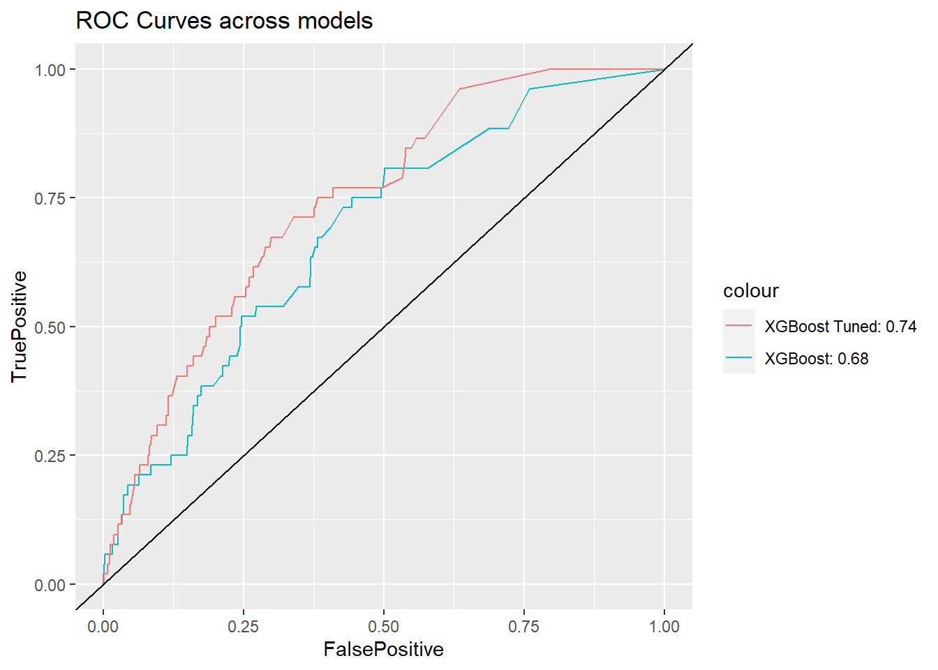
The tuned model AUC is 0.7416419 which is much higher than the model with default paraeters. Yeah, we have improved the model by tuning the parameters.

Lastly, let’s plot the curves.

ROCperf.xgb.tuned <- performance(ROCpred.xgb.tuned, 'tpr','fpr')
df_ROC.xgb_tune <- data.frame(FalsePositive = c(ROCperf.xgb.tuned@x.values[[1]]),
                              TruePositive = c(ROCperf.xgb.tuned@y.values[[1]]))

ggplot() +
  geom_line(data = df_ROC.xgb, aes(x = FalsePositive,
                                   y = TruePositive,
                                   color = "XGBoost: 0.68")) + 
  geom_line(data = df_ROC.xgb_tune, aes(x = FalsePositive,
                                        y = TruePositive,
                                        color = "XGBoost Tuned: 0.74")) + 
  geom_abline(slope = 1) + ggtitle("ROC Curves across models")

Bonus: Parallel computing

You may experience long waiting time when you try to train more complex machine learning models using larger data set. For the optimization process we tried above, it takes more than 3 minutes. But did you know that your computer can run the function simultaneously? Computer CPU has multiple threads/cores which can do parallel computing.

I will demonstrate how we can run parallel computing using the package:doParallel. The package:ParBayesianOptimization also supports parallel computing.

Don’t know how many cores/threads your CPU has? Don’t worry, we can use the detectCores() to find the number. Note that you’d better not use all of your cores to prevent crash of your computer. My computer has 6 cores and 12 threads and I am using half for this example (ie, 6 threads).

To enable the parallel computing, you must meet the following criteria:

• Make a socket cluster for multiple threads/cores working together. This is done by the makeCluster() function.
• A parallel backend must be registered, this is done by the registerDoParallel() function.
• Objects required by FUN must be loaded into each cluster. This will be done by the the clusterExport() function. For our example, the FUN function needs to use the data x and y which are defined outside of the FUN function.
• Packages required by FUN must be loaded into each cluster. This will be done by the the clusterEvalQ() function. For our example, the FUN function needs the package:xgboost as it uses the xgb.DMatrix() function.
• FUN must be thread safe. It means the function can be run simultaneously on multiple threads and the results should be the same as running on one thread serially. For example, each run of the FUN should be independent and one run of FUN is not depend on the previous run of FUN. You may refer more knowledge on thread safe coding here.

In addition, you must enable the parallel = TRUE option in the bayesOpt() function. After done with paralleing computing, you must stop it and continue with serial computing by using the stopCluster() and registerDoSEQ().

Okay, we are ready for the code.

set.seed(2021)

library(doParallel)
no_cores <- detectCores() / 2 # use half my CPU cores to avoid crash  
cl <- makeCluster(no_cores) # make a cluster
registerDoParallel(cl) # register a parallel backend
clusterExport(cl, c('x','y')) # import objects outside
clusterEvalQ(cl,expr= { # launch library to be used in FUN
  library(xgboost)
})

time_withparallel <- system.time(
opt_obj <- bayesOpt(
  FUN = scoring_function,
  bounds = bounds,
  initPoints = 7,
  iters.n = 5,
  parallel = TRUE
))

stopCluster(cl) # stop the cluster
registerDoSEQ() # back to serial computing

The time spent is 52.19 seconds, which is much faster than without parallel computing (193 seconds).

Done!

Thanks for reading this post and I hope you find it useful. It is indeed a very fun process when you are able to get better results.

In sum, we start our model training using the XGBoost default hyperparameters. We then improve the model by tuning six important hyperparameters using the package:ParBayesianOptimization which implements a Bayesian Optimization algorithm. I also demonstrate the parallel computing which significantly saves computing time and resources.

Feel free to try hyperparameter tuning in your group project. Let me know if you have any questions by booking my time at https://calendly.com/drdataking.

This post is a supplementary reading to the SMU Master of Professional Accounting program' elective course Programming with Data.

Last updated on 07 November, 2021